The CUDA Handbook ▸ Chapter 15. Image Processing: Normalized Correlation

15.8 The Denominator: Summed Area Tables

Regardless how the numerators are computed, every coefficient also needs a denominator, which for every \(T \times T\) region, requires the image’s first and second moments: \(\sum I\) and \(\sum I^2\). Computed directly, each is \(O(K)\) per output pixel, the very per-pixel cost the numerator methods work to avoid.

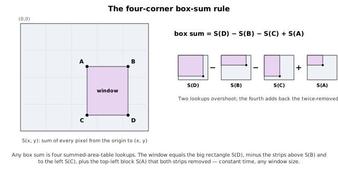
To replace this \(O(K)\) operation with a constant-time lookup, Lewis introduced an intermediate data structure called the summed-area table (SAT). The table – introduced by Franklin Crow for texture antialiasing – holds at \(S(x,y)\) the sum of every pixel above and to the left of \((x,y)\), so the sum over any rectangle is a four-corner difference,

\[\sum_{[x_0, x_1) \times [y_0, y_1)} I = S(x_1{-}1, y_1{-}1) - S(x_0{-}1, y_1{-}1) - S(x_1{-}1, y_0{-}1) + S(x_0{-}1, y_0{-}1),\]

computed in constant time regardless of the window size. One table serves every window, every template in a bank, and every shift in an FFT search; a second SAT, built the same way on the squared pixels, supplies \(\sum I^2\).

Figure 15-7. The four-corner box-sum rule.

The query is four loads and three adds, valid on both the host and the device – the corners named as in Figure 15-7, with the two edges of the SAT treated as zero:

__host__ __device__ int64_t
satBox( const int64_t *S, int W, int x0, int y0, int x1, int y1 )
{
    int64_t D =                  S[(y1-1)*W + (x1-1)];      // bottom-right
    int64_t B = (y0>0)         ? S[(y0-1)*W + (x1-1)] : 0;  // top-right
    int64_t C = (x0>0)         ? S[(y1-1)*W + (x0-1)] : 0;  // bottom-left
    int64_t A = (x0>0 && y0>0) ? S[(y0-1)*W + (x0-1)] : 0;  // top-left
    return D - B - C + A;
}

The table must be built in a wide enough type. The whole-image sum of an 8-bit image reaches \(WH \cdot 255\), and the sum of squares reaches \(WH \cdot 255^2\), which passes \(2^{31}\) by a 512×512 image; the table is therefore int64. Since each row’s running sum is much smaller, at most \(W \cdot 255^2\), we can store those as uint32, halving the memory traffic of the build. Only the final table needs the full width.

Building the table, not querying it, is the expensive part. A naive one-thread-per-line build of both tables takes about 6.8 ms at 4096×4096 on a GeForce RTX 3060 – more than the FFT numerator it serves. It is separable and simple, one thread per row and then one thread per column, computing both moments at once:

// row pass: each thread runs one row's inclusive scan
__global__ void
naiveRow( const uint8_t *img, int W, int H, int64_t *S, int64_t *Q )
{
    for ( int y = blockIdx.x*blockDim.x + threadIdx.x; y < H;
              y += gridDim.x*blockDim.x ) {
        int64_t sum = 0, sqsum = 0;
        for ( int x = 0; x < W; x++ ) {
            int v = img[y*W + x];
            sum   += v;
            sqsum += v*v;
            S[y*W + x] = sum;      // running sum of pixels
            Q[y*W + x] = sqsum;    // running sum of squares
        }
    }
}

// column pass: each thread runs one column's inclusive scan over the row sums
__global__ void
naiveCol( int W, int H, int64_t *S, int64_t *Q )
{
    for ( int x = blockIdx.x*blockDim.x + threadIdx.x; x < W;
              x += gridDim.x*blockDim.x ) {
        int64_t sum = 0, sqsum = 0;
        for ( int y = 0; y < H; y++ ) {
            sum   += S[y*W + x];
            sqsum += Q[y*W + x];
            S[y*W + x] = sum;
            Q[y*W + x] = sqsum;
        }
    }
}

Each thread writes an output row or column, and naiveCol strides through memory by the row width with no reuse – which is why it is the slow baseline, the SAT_NAIVE build.

A summed-area table is separable, though – an inclusive scan along each row, then down each column – and a scan is exactly what a library provides. cub::DeviceScan runs the row scans with the single-pass decoupled look-back of Merrill and Garland (Chapter 13). CUB’s Scan only works on contiguous memory, though, so the algorithm must scan the rows, transpose, scan the now-columns, and transpose again. That two-transpose library build is SAT_CUB, several times faster than the naive one; but for an int64 table, those two transposes move more memory than the scans themselves.

We can eliminate the need for the transposes with a purpose-built column scan (Figure 15-8). Because the SAT columns are independent, a single-pass decoupled look-back can scan them in place: each block owns a strip of columns and a stripe of rows, publishes its per-column partial sums, and looks back over earlier stripes for the running carry. That transpose-free build is SAT_DLB; on the RTX 3060, building both tables at 4096×4096, it runs about 3× faster than SAT_CUB and more than 3× faster than SAT_NAIVE.

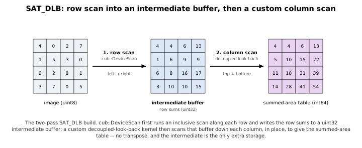
Figure 15-8. The two-pass SAT_DLB build: a cub::DeviceScan of the rows writes an intermediate buffer, then a custom decoupled-look-back scan runs down its columns to produce the table.

With some additional accounting, the decoupled look-back can be extended to two dimensions, eliminating the uint32 intermediate. Each block stages one tile in shared memory, scans its rows with a horizontal look-back over the tiles to its left, then scans its columns with a vertical look-back over the tiles above. Furthermore, both moments are computed in the same pass, so the image data is loaded just once. Handing the tiles out in row-major order keeps every dependence pointing at an earlier tile, so the two look-backs cannot deadlock. On the RTX 3060, building both tables at 4096×4096, SAT_FUSED runs about 1.9× faster than SAT_DLB (1.09 ms versus 2.06 ms), about 5.7× faster than SAT_CUB, and about 6× faster than SAT_NAIVE – with the whole-image intermediate now gone.

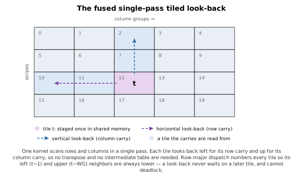
Figure 15-9. The fused single-pass tiled look-back.

Each carry is a decoupled look-back along one axis (Figure 15-9), gathering a tile’s carry from its neighbors – to the left for the row scan, above for the column scan. A three-state flag per tile carries the protocol: a tile publishes its own aggregate (state 1), then its finished prefix (state 2) once it has looked back; a neighbor reading it takes the prefix if it is ready and stops, or adds the aggregate and keeps looking further back. Here’s an excerpt from the horizontal pass (the vertical pass is the same idea rotated ninety degrees):

// horizontal look-back: gather this row's carry from the tiles to its left.
// statusH[]: 0 = not ready, 1 = aggregate published, 2 = full prefix published.
uint32_t carry = 0;
for ( int p = colGroup - 1; p >= 0; p-- ) {
    int prev = stripe*WG + p;
    int st = statusH[prev];

    // spin until the neighbor publishes
    while ( 0 == st ) st = statusH[prev];    
    __threadfence();
    if ( 2 == st ) {
        // its prefix is final: take it and stop
        carry += rowPref[prev*SAT_BR + row];
        break;
    }
    carry += rowAgg[prev*SAT_BR + row];      // only an aggregate so far: keep going
}

Because tiles are handed out in row-major order, the look-back only ever waits on lower-numbered tiles, so cannot deadlock.

The summed-area table, its four builds – SAT_NAIVE, SAT_CUB, SAT_DLB, and SAT_FUSED – and the four-corner query are implemented in sat.cuh; integralImage.cu drives them and reports the build times above.