All texture intrinsics except tex1Dfetch() use floating point values
to specify coordinates into the texture. When using unnormalized
coordinates, they fall in the range [0, MaxDim) where
MaxDim is the width, height or depth of the texture.
Unnormalized coordinates are an intuitive way to index into a texture,
but some texturing features are not available when using them.
An easy way to study texturing behavior is to populate a texture with
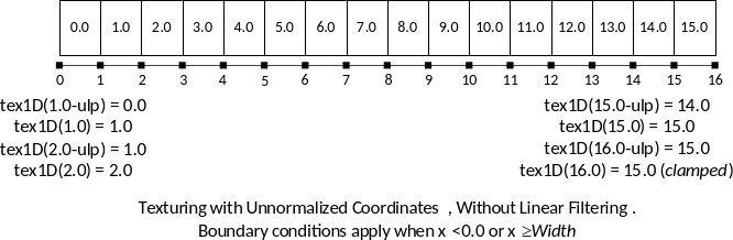
elements that contain the index into the texture. Figure 10-4 shows a
float-valued 1D texture with 16 elements, populated by the identity
elements and annotated with some sample values returned by tex1D().
Figure 10-4. Texturing with Unnormalized Coordinates (without linear filtering)
template<class T>voidCreateAndPrintTex( T *initTex, size_t texN, size_t outN, float base, float increment, cudaTextureFilterMode filterMode = cudaFilterModePoint, cudaTextureAddressMode addressMode = cudaAddressModeClamp ){ T *texContents = 0; cudaArray *texArray = 0; float2 *outHost = 0, *outDevice = 0; cudaError_t status; cudaChannelFormatDesc channelDesc = cudaCreateChannelDesc<T>(); // use caller-provided array, if any, to initialize texture if ( initTex ) { texContents = initTex; } else { // default is to initialize with identity elements texContents = (T *) malloc( texN*sizeof(T) ); if ( ! texContents ) goto Error; for ( int i = 0; i < texN; i++ ) { texContents[i] = (T) i; } } cuda(MallocArray(&texArray, &channelDesc, texN)); cuda(HostAlloc( (void **) &outHost, outN*sizeof(float2), cudaHostAllocMapped)); cuda(HostGetDevicePointer( (void **) &outDevice, outHost, 0 )); cuda(MemcpyToArray( texArray, 0, 0, texContents, texN*sizeof(T), cudaMemcpyHostToDevice)); cuda(BindTextureToArray(tex, texArray)); tex.filterMode = filterMode; tex.addressMode[0] = addressMode; cuda(HostGetDevicePointer(&outDevice, outHost, 0)); TexReadout<<<2,384>>>( outDevice, outN, base, increment ); cuda(DeviceSynchronize()); for ( int i = 0; i < outN; i++ ) { printf( "(%.2f, %.2f)\n", outHost[i].x, outHost[i].y ); } printf( "\n" ); Error: if ( ! initTex ) free( texContents ); if ( texArray ) cudaFreeArray( texArray ); if ( outHost ) cudaFreeHost( outHost );}tex1d_unnormalized.cu (excerpt) (source on GitHub)Not all texturing features are available with unnormalized coordinates, but they can be used in conjunction with linear filtering and a limited form of texture addressing.
The texture addressing mode specifies how the hardware should deal with out-of-range texture coordinates. For unnormalized coordinates, the above figure illustrates the default texture addressing mode of clamping to the range [0, MaxDim) before fetching data from the texture: the value 16.0 is out of range, and clamped to fetch the value 15.0. Another texture addressing option available when using unnormalized coordinates is the “border” addressing mode, where out-of-range coordinates return zero.
The default filtering mode, so-called “point filtering,” returns one
texture element depending on the value of the floating-point coordinate.
In contrast, linear filtering causes the texture hardware to fetch the
two neighboring texture elements and linearly interpolate between them,
weighted by the texture coordinate. The below figure shows the 1D
texture with 16 elements, with some sample values returned by tex1D().
Note that you must add 0.5f to the texture coordinate to get the
identity element.
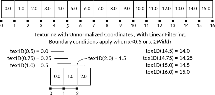
Figure 10-5. Texturing with Unnormalized Coordinates (with linear filtering)
Many texturing features can be used in conjunction with one another;
for example, linear filtering can be combined with the
previously-discussed promotion from integer to floating point. In that
case, the floating point outputs produced by tex1D() intrinsics are
accurate interpolations between the promoted floating-point values of
the two participating texture elements.
tex1d_unnormalized.cuThe microdemo tex1d_unnormalized.cu is like a microscope to closely
examine texturing behavior by printing the coordinate and the value
returned by the tex1D() intrinsic together. Unlike the
tex1dfetch_int2float.cu microdemo, this program uses a 1D CUDA array to
hold the texture data. Some number of texture fetches is performed,
along a range of floating point values specified by a base and
increment; the interpolated values and the value returned by tex1D() are
written together into an output array of float2. The CUDA kernel is as
follows:
extern "C" __global__ void
TexReadout( float2 *out, cudaTextureObject_t tex, size_t N, float base, float increment )
{
    for ( size_t i = blockIdx.x*blockDim.x + threadIdx.x;
          i < N;
          i += gridDim.x*blockDim.x )
    {
        float x = base + (float) i * increment;
        out[i].x = x;
        out[i].y = tex1D<float>( tex, x );
    }
}
A host function CreateAndPrintTex() takes the size of the texture to
create, the number of texture fetches to perform, the base and increment
of the floating point range to pass to tex1D(), and optionally the
filter and addressing modes to use on the texture. This function creates
the CUDA array to hold the texture data, optionally initializes it with
the caller-provided data (or identity elements if the caller passes
NULL), creates a texture object over the CUDA array with the requested
filter and addressing modes, and prints the float2 output.
The main() function for this program is intended to be modified to
study texturing behavior. This version creates an 8-element texture and
writes the output of tex1D() from 0.0 .. 7.0:
int
main( int argc, char *argv[] )
{
    cudaError_t status;
    cuda(SetDeviceFlags(cudaDeviceMapHost));
    CreateAndPrintTex<float>( NULL, 8, 8, 0.0f, 1.0f );
    CreateAndPrintTex<float>( NULL, 8, 8, 0.0f, 1.0f, cudaFilterModeLinear );
    return 0;
}
The output from this program is as follows:
(0.00, 0.00)    <- output from the first CreateAndPrintTex()
(1.00, 1.00)
(2.00, 2.00)
(3.00, 3.00)
(4.00, 4.00)
(5.00, 5.00)
(6.00, 6.00)
(7.00, 7.00)
(0.00, 0.00)    <- output from the second CreateAndPrintTex()
(1.00, 0.50)
(2.00, 1.50)
(3.00, 2.50)
(4.00, 3.50)
(5.00, 4.50)
(6.00, 5.50)
(7.00, 6.50)
If we change main() to invoke CreateAndPrintTex() as follows:
CreateAndPrintTex<float>( NULL, 8, 20, 0.9f, 0.01f, cudaFilterModePoint );
The resulting output highlights that when point filtering, 1.0 is the dividing line between texture elements 0 and 1:
(0.90, 0.00)
(0.91, 0.00)
(0.92, 0.00)
(0.93, 0.00)
(0.94, 0.00)
(0.95, 0.00)
(0.96, 0.00)
(0.97, 0.00)
(0.98, 0.00)
(0.99, 0.00)
(1.00, 1.00)    <- transition point
(1.01, 1.00)
(1.02, 1.00)
(1.03, 1.00)
(1.04, 1.00)
(1.05, 1.00)
(1.06, 1.00)
(1.07, 1.00)
(1.08, 1.00)
(1.09, 1.00)
One limitation of linear filtering is that it is performed with 9-bit
weighting factors. It is important to realize that the precision of the
interpolation depends, not on that of the texture elements, but on the
weights. As an example, let’s take a look at a 10-element texture
initialized with normalized identity elements, i.e. (0.0, 0.1, 0.2, 0.3,
… 0.9) instead of (0, 1, 2, … 9). CreateAndPrintTex() lets us specify
the texture contents, so we can do so as follows:
    {
        float texData[10];
        for ( int i = 0; i < 10; i++ ) {
            texData[i] = (float) i / 10.0f;
        }
        CreateAndPrintTex<float>( texData, 10, 10, 0.0f, 1.0f );
    }
The output from an unmodified CreateAndPrintTex() looks innocuous
enough:
(0.00, 0.00)
(1.00, 0.10)
(2.00, 0.20)
(3.00, 0.30)
(4.00, 0.40)
(5.00, 0.50)
(6.00, 0.60)
(7.00, 0.70)
(8.00, 0.80)
(9.00, 0.90)
Or, if we invoke CreateAndPrintTex() with linear interpolation
between the first two texture elements (values 0.1 and 0.2):
CreateAndPrintTex<float>(tex,10,10,1.5f,0.1f,cudaFilterModeLinear);
The resulting output is as follows:
(1.50, 0.10)
(1.60, 0.11)
(1.70, 0.12)
(1.80, 0.13)
(1.90, 0.14)
(2.00, 0.15)
(2.10, 0.16)
(2.20, 0.17)
(2.30, 0.18)
(2.40, 0.19)
Rounded to 2 decimal places, this data looks very well behaved. But
if we modify CreateAndPrintTex() to output hexadecimal instead, the
output becomes:
(1.50, 0x3dcccccd)
(1.60, 0x3de1999a)
(1.70, 0x3df5999a)
(1.80, 0x3e053333)
(1.90, 0x3e0f3333)
(2.00, 0x3e19999a)
(2.10, 0x3e240000)
(2.20, 0x3e2e0000)
(2.30, 0x3e386667)
(2.40, 0x3e426667)
It is clear that most fractions of 10 are not exactly representable in floating point. Nevertheless, when performing interpolation that does not require high precision, these values are interpolated at full precision.
tex1d_9bit.cuTo explore this question of precision, we developed another
microdemo, tex1d_9bit.cu. Here, we’ve populated a texture
with 32-bit floating point values that require full precision to
represent. In addition to passing the base/increment pair for the
texture coordinates, another base/increment pair specifies the
“expected” interpolation value, assuming full-precision
interpolation.
In tex1d_9bit, the CreateAndPrintTex() function is
modified to write its output as shown in Listing 10-3.
printf( "X\tY\tActual Value\tExpected Value\tDiff\n" );for ( int i = 0; i < outN; i++ ) { T expected; if ( bEmulateGPU ) { float x = base+(float)i*increment - 0.5f; float frac = x - (float) (int) x; { int frac256 = (int) (frac*256.0f+0.5f); frac = frac256/256.0f; } int index = (int) x; expected = (1.0f-frac)*initTex[index] + frac*initTex[index+1]; } else { expected = expectedBase + (float) i*expectedIncrement; } float diff = fabsf( outHost[i].y - expected ); printf( "%.2f\t%.2f\t", outHost[i].x, outHost[i].y ); printf( "%08x\t", *(int *) (&outHost[i].y) ); printf( "%08x\t", *(int *) (&expected) ); printf( "%E\n", diff );}printf( "\n" );Tex1d_9bit.cu (excerpt) (source on GitHub)For the just-described texture with 10 values (incrementing by 0.1), we can use this function to generate a comparison of the actual texture results with the expected full-precision result. Calling the function:
CreateAndPrintTex<float>( tex, 10, 4, 1.5f, 0.25f, 0.1f, 0.025f );
CreateAndPrintTex<float>( tex, 10, 4, 1.5f, 0.1f, 0.1f, 0.01f );
yields this output:
X     Y     Actual Value    Expected Value  Diff
1.50  0.10  3dcccccd        3dcccccd        0.000000E+00
1.75  0.12  3e000000        3e000000        0.000000E+00
2.00  0.15  3e19999a        3e19999a        0.000000E+00
2.25  0.17  3e333333        3e333333        0.000000E+00

X     Y     Actual Value    Expected Value  Diff
1.50  0.10  3dcccccd        3dcccccd        0.000000E+00
1.60  0.11  3de1999a        3de147ae        1.562536E-04
1.70  0.12  3df5999a        3df5c290        7.812679E-05
1.80  0.13  3e053333        3e051eb8        7.812679E-05
As you can see from the “Diff” column on the right, the first set of outputs were interpolated at full-precision, while the second were not. The explanation for this difference lies in Appendix F of the CUDA Programming Guide, which describes how linear interpolation is performed for 1D textures:
\[tex(x) = (1 - \propto )T(i) + \propto T(i + 1)\]
where:
\[i = floor\left( X_{B} \right),\ \propto = frac\left( X_{B} \right),\ X_{B} = x - 0.5\]
and α is stored in a 9-bit fixed-point format with 8 bits of fractional value.
In Listing 10-3, this computation in C++ is emulated in the
bEmulateGPU case.
The code snippet to emulate 9-bit weights can be enabled in
tex1d_9bit.cu by passing true as the
bEmulateGPU parameter of CreateAndPrintTex(). The output
then becomes:
X     Y     Actual Value    Expected Value  Diff
1.50  0.10  3dcccccd        3dcccccd        0.000000E+00
1.75  0.12  3e000000        3e000000        0.000000E+00
2.00  0.15  3e19999a        3e19999a        0.000000E+00
2.25  0.17  3e333333        3e333333        0.000000E+00

X     Y     Actual Value    Expected Value  Diff
1.50  0.10  3dcccccd        3dcccccd        0.000000E+00
1.60  0.11  3de1999a        3de1999a        0.000000E+00
1.70  0.12  3df5999a        3df5999a        0.000000E+00
1.80  0.13  3e053333        3e053333        0.000000E+00
As you can see from the rightmost column of 0’s, when computing the interpolated value with 9-bit precision, the differences between “expected” and “actual” output disappear.