The author wishes to thank Sean Baxter, Duane Merrill, and Lars Nyland for their help in preparing this chapter.
If you were trying to characterize a set of M&M candies, one of the more obvious ways to do so would be to examine each candy and record its color. According to Wikipedia, there have been eight (8) colors of M&M over the decades: blue, brown, green, orange, red, tan, violet, and yellow. If you start with 8 counters – one for each color – and for each candy increment the counter corresponding to the color of the candy, you will have constructed a histogram: a statistical function that counts the number of observations that fall into each of some number of discrete categories. An oft-used metaphor for histograms is to say that each input element got put into a specific bin; in the case of M&M candies, there would be 8 bins, and after processing some set of M&Ms, the histogram would be represented by the number of candies in each bin. Histograms are often depicted as graphical representations of the data distribution, but for computers, a histogram usually consists of an array of k integers, where k is the number of bins; in the case of our M&M candy example, k==8. After accumulating N observations, the sum of the k integers is equal to N.
As an example, I recorded the colors of the 24 M&M’s from a bag (for the sake of simplicity, only 7 colors are represented since blue and brown start with the same letter):
BOYRGBYRVYOBVBYGRVVBBGGR
With one bucket per possible color, Table 16-1 gives the counts. Note that in this random sample of candies, there were no tan candies, so the T count is 0.
| Color | Count |
|---|---|
| B | 6 |
| G | 4 |
| O | 2 |
| R | 4 |
| T | 0 |
| V | 4 |
| Y | 4 |
Table 16-1. Number of candies by color
If k is much smaller than N, as with our colored candies (i.e. the number of possible colors (8) usually is much smaller than the number of candies), then an array of k integers (one for each of the k categories) is a suitable representation for a histogram.
Histograms have many applications. For statisticians, they help to visualize the central location(s), spread, and shape of the input data. Histograms can be used to compute order statistics (e.g. a selected element in the sorted order of the input data – the most famous is the median or middle element), though such methods are best used if a histogram was needed for other reasons. Other statistics, such as the total number of samples (just compute the sum of the histogram bins) or the mean of the samples, also are easily computed using the histogram. In image processing, the peaks and valleys of the histogram can be used for thresholding (i.e. to select a value or values that would be suitable for reducing the bit depth, e.g. to convert the image to a binary representation) for edge detection or image segmentation.
A final application of histograms that deserves mention is counting sort: if the k bins in the histogram are in sorted order, you can emit a sorted list by sweeping across the histogram bins [0..k-1] and using the count in the histogram bin to emit that number of elements. For our example of 24 candies, we can use the histogram to emit the following array, sorted in order of candy color:
BBBBBBGGGGOORRRRVVVVYYYY
This sort is not done by sorting the array per se, but by simply printing B six times (since the histogram element for B is 6), then G four times (since the G histogram element is 4), and so on. If each histogram element can be processed in constant time, counting sort runs in O(N) time. Because it does not compare elements, counting sort is not subject to the minimum asymptotic O(NlgN) runtime of comparison-based sorting algorithms.
Counting sort harkens to an alternative solution to computing the histogram, one that is suitable when N is much smaller than k (for example, if N is the number of transactions by a customer and k is the number of items available from an electronic retailer): sort the N inputs and look for adjacent duplicates (“reduce-by-key”) to identify the number of elements that belong in each bin of the (sparse) histogram.
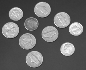
Histograms of any number of elements can be of interest, but for purposes of this chapter, we will focus on the special case of 256 elements, which is important for image processing of 8-bit images. Figure 16-1 shows coins.pgm, the image used in Chapter 15 to illustrate normalized cross-correlation.
Figure 16-1. coins.pgm
Figure 16-2 shows the histogram for coins.pgm. The
histogram has two “spikes” that roughly correspond to the “background”
and “coins.” An image processing algorithm could “binarize” the image by
replacing each pixel with a 0 or 1, depending on whether the pixel value
was above or below a threshold selected by analyzing the histogram.
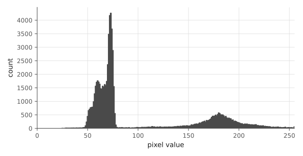
Figure 16-2. Histogram (coins.pgm)
For this image and histogram, a value around 100 works; the resulting black-and-white image is given in Figure 16-3.
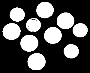
Figure 16-3. coins.pgm (binarized with threshold of
100)
For the remainder of this chapter, we will focus on 256-element histograms of 8-bit input data. For clarity, the code will not use texturing or 2D pitch memory (though such code is included in the sample code on GitHub). Listing 16-1 gives the C code to compute a histogram: the output array is initialized to zero, then for each input element, the corresponding histogram element is incremented.
voidhist1DCPU( unsigned int *pHist, unsigned char *p, size_t N ){ memset( pHist, 0, 256*sizeof(unsigned int) ); for ( size_t i = 0; i < N; i++ ) { pHist[ p[i] ] += 1; }}When parallelizing the histogram computation, there are two basic strategies:
multiple threads update a histogram concurrently, and
compute multiple histograms, then merge them together into the final output.
On CPUs, the OS and hardware support for multithreading make the
first approach prohibitively expensive, whether acquiring and releasing
an OS mutex per histogram element or directly invoking atomic operations
(such as those exposed by C++ std::atomic). In contrast, 2)
could be implemented with a simple fork/join idiom that divided the
problem size evenly among threads (say 1-2 threads per CPU core), then
computed the final output after waiting on the child threads1.
For very small problem size, the overhead of delegating and then waiting on the work might present a problem.↩︎