We arrived at three (3) implementations of 8-bit histogram computation: naïve global atomics that accumulate directly into the final output (“histogram per grid”); per-block histograms that use shared memory atomics (“histogram per block”); and privatized histograms with periodic merge (“histogram per thread”).
All implementations benefited from using 32-bit memory operations to read the input, and unrolling the inner loop 4x in the spirit of Listing 16-3. Therefore, all of the performance results reported here reflect this optimization.
We ran the kernels on large inputs (at least 4096x4096) with the
--random parameter varying from 256 (any 8-bit value may appear in the
input) to 1 (the input data is all 0’s). By decreasing the number of
possible values in the input, we highlight how vulnerable each approach
is to data-dependent performance degradation due to contention. The
privatized histogram-per-thread approach is designed to have level
performance, but does not work well on modern hardware.
The charts that follow (Figures 16-7 through 16-9) are the original measurements on GT200, GF100, and GK104 parts, preserved here as a historical record of how the three approaches compared across the SM 1.x-3.x architectures. Refreshed per-kernel throughput for a current (Ampere) GPU appears in Tables 16-2 through 16-4.
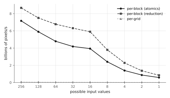
Figure 16-7 shows the results for a GT200 (SM 1.3). Since SM 1.x hardware does not have enough shared memory to run the privatized per-thread algorithm, we report the performance of per-grid, per-block using atomics to accumulate into the final output, and per-block using reduction to accumulate into the final output. (This strategy does not benefit SM 2.x or SM 3.x hardware, due to faster global atomics.) The per-grid implementation that uses global atomics to operate on the output histogram is so slow that its relative performance is impossible to make out from the chart – to get an idea of the relative performance, see Table 16-3.
Figure 16-7. Histogram Performance – SM 1.3
Figure 16-8 shows the results for a GF100 (SM 2.0). The per-thread implementation is level at about 9 billion pixels per second; the per-block implementation is faster for 256 and 128 possible values, but crosses over at 64 possible values and rapidly degrades from there. The per-grid implementation appears on the chart, but is uncompetitive for all possible input values.
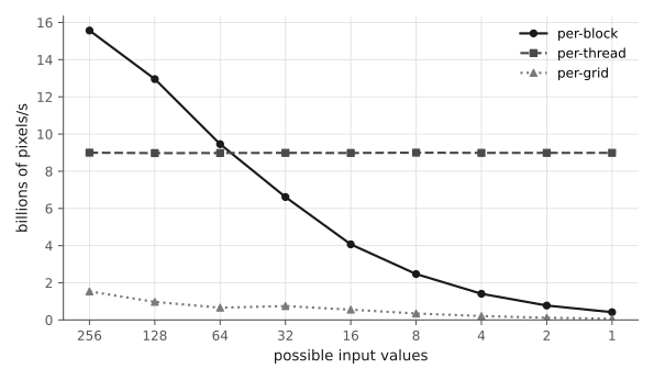
Figure 16-8. Histogram Performance – SM 2.0
Figure 16-9 shows the results for a GK104 (SM 3.0). Here, the per-grid performance is much more competitive – it is actually faster than the per-thread implementation for 256 possible input values – but the most noteworthy result is that GK104 runs the per-thread implementation significantly slower than the older GF100! (About 6.6 billion pixels per second versus 9 billion pixels per second.) The two architectures are extremely different – Kepler has fewer SMs and more execution units per SM – and the low-occupancy structure of the per-thread kernel is not a great architectural fit for Kepler. Unfortunately, neither the per-grid nor the per-block formulations are.
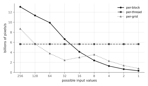
Figure 16-9. Histogram Performance – SM 3.0