Fast native floating point hardware is the raison d’etre for GPUs, and in many ways they are equal to or superior to CPUs in their floating point implementation. Denormals are supported at full speed10, directed rounding may be specified on a per-instruction basis, and the Special Function Units deliver high-performance approximation functions to six popular single-precision transcendentals. In contrast, x86 CPUs implement denormals in microcode that runs perhaps 100x slower than operating on normalized floating point operands; rounding direction is specified by a control word that takes dozens of clock cycles to change; and the only transcendental approximation functions in the SSE instruction set are for reciprocal and reciprocal square root, which give 12-bit approximations that must be refined with a Newton-Raphson iteration before being used.
Since GPUs’ greater core counts are offset somewhat by their lower clock frequencies, developers can expect at most a 10x (or thereabouts) speedup on a level playing field. If a paper reports a 100x or greater speedup from porting an optimized CPU implementation to CUDA, chances are one of the above-described “instruction set mismatches” played a role.
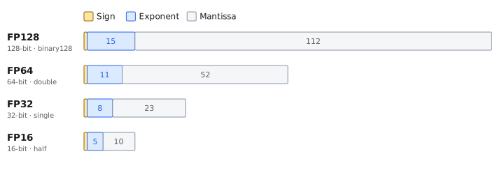
Figure 8-2 depicts the IEEE standard floating point formats CUDA supports, from half precision (16-bit) up to quadruple precision (128-bit). For its first decade, CUDA offered only double, single, and half; the deep learning era has since added a family of narrower formats (Section 8.3.5, Figure 8-3), while quadruple precision—new, and software-emulated—extends the range in the other direction. Each value is divided into three fields: sign, exponent, and mantissa. For half, single, double and quad, the exponent fields are 5, 8, 11 and 15 bits in size, respectively; the corresponding mantissa fields are 10, 23, 52 and 112 bits.
Figure 8-2. Floating Point Formats
The exponent field changes the interpretation of the floating point value. The most common (“normal”) representation encodes an implicit 1 bit into the mantissa, and multiplies that value by 2e-bias, where bias is the value added to the actual exponent before encoding into the floating point representation. The bias for single precision, for example, is 127.
Table 8-7 summarizes how floating-point values are encoded. For most exponent values (so-called “normal” floating-point values), the mantissa is assumed to have an implicit 1, and is multiplied by the biased value of the exponent. The maximum exponent value is reserved for infinity and Not-A-Number values. Dividing by zero (or overflowing a division) yields infinity; performing an invalid operation (such as taking the square root or logarithm of a negative number) yields a NaN. The minimum exponent value is reserved for values too small to represent with the implicit leading 1: as the so-called denormals11 get closer to zero, they lose bits of effective precision, a phenomenon known as gradual underflow.
Table 8-8 gives the encodings and values of certain extreme values for each format.
| Exponent | Mantissa | Value | Case Name |
|---|---|---|---|
| Quadruple precision | |||
| 0 | 0 | ±0 | Zero |
| 0 | Nonzero | ±2-16382(0.mantissa) | Denormal |
| 1 to 32766 | Any | ±2e-16383(1.mantissa) | Normal |
| 32767 | 0 | ±∞ | Infinity |
| 32767 | Nonzero | Not a number | |
| Double precision | |||
| 0 | 0 | ±0 | Zero |
| 0 | Nonzero | ±2-1022(0.mantissa) | Denormal |
| 1 to 2046 | Any | ±2e-1023(1.mantissa) | Normal |
| 2047 | 0 | ±∞ | Infinity |
| 2047 | Nonzero | Not a number | |
| Single precision | |||
| 0 | 0 | ±0 | Zero |
| 0 | Nonzero | ±2-126(0.mantissa) | Denormal |
| 1 to 254 | Any | ±2e-127(1.mantissa) | Normal |
| 255 | 0 | ±∞ | Infinity |
| 255 | Nonzero | Not a number | |
| Half precision | |||
| 0 | 0 | ±0 | Zero |
| 0 | Nonzero | ±2-14(0.mantissa) | Denormal |
| 1 to 30 | Any | ±2e-15(1.mantissa) | Normal |
| 31 | 0 | ±∞ | Infinity |
| 31 | Nonzero | Not a number |
Table 8-7. Floating Point Representations
| Hexadecimal | Exact value | |
|---|---|---|
| Quadruple precision | ||
| Smallest denormal | 0...01 |
2-16494 |
| Largest denormal | 0000 F...F |
2-16382(1-2-112) |
| Smallest normal | 0001 0...0 |
2-16382 |
| 1.0 | 3FFF 0...0 |
1 |
| Maximum integer | 4070 0...0 |
2113 |
| Largest normal | 7FFE F...F |
216384(1-2-113) |
| Infinity | 7FFF 0...0 |
Infinity |
| Double precision | ||
| Smallest denormal | 0...0001 |
2-1074 |
| Largest denormal | 000F...F |
2-1022(1-2-52) |
| Smallest normal | 0010...0 |
2-1022 |
| 1.0 | 3FF0...0 |
1 |
| Maximum integer | 4340...0 |
253 |
| Largest normal | 7FEF...F |
21024(1-2-53) |
| Infinity | 7FF0...0 |
Infinity |
| Single precision | ||
| Smallest denormal | 00000001 |
2-149 |
| Largest denormal | 007FFFFF |
2-126(1-2-23) |
| Smallest normal | 00800000 |
2-126 |
| 1.0 | 3F800000 |
1 |
| Maximum integer | 4B800000 |
224 |
| Largest normal | 7F7FFFFF |
2128(1-2-24) |
| Infinity | 7F800000 |
Infinity |
| Half precision | ||
| Smallest denormal | 0001 |
2-24 |
| Largest denormal | 07FF |
2-14(1-2-10) |
| Smallest normal | 0800 |
2-14 |
| 1.0 | 3c00 |
1 |
| Maximum integer | 6800 |
211 |
| Largest normal | 7BFF |
216(1-2-11) |
| Infinity | 7C00 |
Infinity |
Table 8-8. Floating Point Extreme Values
Quadruple precision (__float128) is the newest and most
unusual of these formats. GPUs have no 128-bit floating point hardware,
so CUDA emulates it in software: the __nv_fp128_ routines
in
crt/device_fp128_functions.h—__nv_fp128_sqrt(),
__nv_fp128_sin(), and the rest—build IEEE binary128
arithmetic out of integer operations. It is far slower than the hardware
formats and is not meant for bulk computation; its purpose is the
occasional extended-precision calculation—a trustworthy reference
result, or an ill-conditioned reduction—where double’s 53
bits of significand are not enough. With 15 exponent bits and 112
mantissa bits (bias 16383), it spans roughly ±1.19×104932 and
carries about 34 decimal digits of precision.
The IEEE standard provides for four (4) round modes:
round-to-nearest-even (also called “round-to-nearest”),
round toward zero (also called “truncate” or “chop”),
round down (or “round toward negative infinity”),
round up (or “round toward positive infinity”).
Round-to-nearest, where intermediate values are rounded to the nearest representable floating point value after each operation, is by far the most commonly used round mode. Round up and round down (the “directed rounding modes”) are used for interval arithmetic, where a pair of floating point values are used to bracket the intermediate result of a computation. To correctly bracket a result, the lower and upper values of the interval must be rounded toward negative infinity (“down”) and toward positive infinity (“up”), respectively.
The C language does not provide any way to specify round modes on a per-instruction basis, and CUDA hardware does not provide a control word to implicitly specify rounding modes. Consequently, CUDA provides a set of intrinsics to specify the round mode of an operation, as summarized in Table 8-9.
| Intrinsic | Operation |
|---|---|
__fadd_[rn|rz|ru|rd] |
Addition |
__fmul_[rn|rz|ru|rd] |
Multiplication |
__fmaf_[rn|rz|ru|rd] |
Fused multiply-add |
__frcp_[rn|rz|ru|rd] |
Reciprocal |
__fdiv_[rn|rz|ru|rd] |
Division |
__fsqrt_[rn|rz|ru|rd] |
Square root |
__dadd_[rn|rz|ru|rd] |
Addition |
__dmul_[rn|rz|ru|rd] |
Multiplication |
__fma_[rn|rz|ru|rd] |
Fused multiply-add |
__drcp_[rn|rz|ru|rd] |
Reciprocal |
__ddiv_[rn|rz|ru|rd] |
Division |
__dsqrt_[rn|rz|ru|rd] |
Square root |
Table 8-9. Intrinsics for Rounding
In general, developers can convert between different floating-point representations and/or integers using standard C constructs: implicit conversion or explicit typecasts. If necessary, however, developers can use the intrinsics listed in Table 8-10 to perform conversions that are not in the C language specification, such as ones with directed rounding.
| Intrinsic | Operation |
|---|---|
__float2int_[rn|rz|ru|rd] |
float to int |
__float2uint_[rn|rz|ru|rd] |
float to unsigned int |
__int2float_[rn|rz|ru|rd] |
int to float |
__uint2float_[rn|rz|ru|rd] |
unsigned int to float |
__float2ll_[rn|rz|ru|rd] |
float to 64-bit int |
__ll2float_[rn|rz|ru|rd] |
64-bit int to float |
__ull2float_[rn|rz|ru|rd] |
64-bit unsigned int to float |
__double2float_[rn|rz|ru|rd] |
double to float |
__double2int_[rn|rz|ru|rd] |
double to int |
__double2uint_[rn|rz|ru|rd] |
double to unsigned int |
__double2ll_[rn|rz|ru|rd] |
double to 64-bit int |
__double2ull_[rn|rz|ru|rd] |
double to 64-bit unsigned int |
__int2double_rn |
int to double |
__uint2double_rn |
unsigned int to double |
__ll2double_[rn|rz|ru|rd] |
64-bit int to double |
__ull2double_[rn|rz|ru|rd] |
64-bit unsigned int to double |
Table 8-10. Intrinsics for conversion
When this book was first written, half was not a type in
the C language, so CUDA expressed these conversions in terms of
unsigned short. Since CUDA 7.5, the __half
type in cuda_fp16.h (Section 8.3.4) has given the operands
a proper type:
__half __float2half( float );
float  __half2float( __half );
All four IEEE rounding modes are available for the
float-to-half direction through the
__float2half_[rn|rz|ru|rd] family; the plain
__float2half() rounds to nearest even.
Single precision floating point support is the workhorse of GPU
computation: GPUs have been optimized to natively deliver high
performance on this data type12, not only for core
standard IEEE operations such as addition and multiplication, but also
for non-standard operations such as approximations to transcendentals
such as sin() and log(). The 32-bit values are held in the same register
file as integers, so coercion between single precision floating point
values and 32-bit integers (with __float_as_int() and __int_as_float())
is free.
The compiler automatically translates +, - and *operators on floating
point values into addition, multiplication, and multiply-add
instructions. The __fadd_rn() and __fmul_rn() intrinsics may be used to
suppress fusion of addition and multiplication operations into
multiply-add instructions.
On all supported hardware, CUDA’s single-precision division operator
is correctly rounded and IEEE 754-compliant by default. Correct rounding
costs performance, so CUDA also offers a faster, approximate divide,
__fdividef(x,y), which forms the quotient from the SFU’s
reciprocal (Table 8-12). The compiler chooses between them with
--prec-div: the default --prec-div=true emits
the compliant divide, while --prec-div=false—set implicitly
by --use_fast_math—routes division through the fast
path.
Beyond its reduced precision, __fdividef() also gives up
range: for 2126<y<2128 it flushes the result
to zero, and it returns NaN rather than INF
when x is infinite, whereas the compliant divide is correct
across the entire range. Square root is governed the same way, by the
--prec-sqrt flag.
The Special Function Units (SFUs) in the SMs implement fast versions of six common transcendental functions:
sine and cosine,
logarithm and exponential,
reciprocal and reciprocal square root.
The SFUs do not implement full 32-bit precision, but they are reasonably good approximations of these functions (22-24 bits precision – See Table 8-11), and they are fast. For CUDA ports that are significantly faster than an optimized CPU equivalent (say, 25x or more), the code most likely relies on the SFUs.
| Function | Accuracy (good bits) | Ulp error |
|---|---|---|
| \(1/x\) | 24.02 | 0.98 |
| \(1/\sqrt{x}\) | 23.40 | 1.52 |
| \(2^x\) | 22.51 | 1.41 |
| \(\log_2 x\) | 22.57 | n/a |
| \(\sin/\cos\) | 22.47 | n/a |
Table 8-11. SFU accuracy13
The SFUs are accessed with the intrinsics given in Table 8-12.
| Intrinsic | Operation |
|---|---|
__cosf(x) |
\(\cos x\) |
__exp10f(x) |
\(10^{x}\) |
__expf(x) |
\(e^{x}\) |
__fdividef(x,y) |
\(\frac{x}{y}\) |
__logf(x) |
\(\ln x\) |
__log2f(x) |
\(\log_{2}x\) |
__log10f(x) |
\(\log_{10}x\) |
__powf(x,y) |
\(x^{y}\) |
__sinf(x) |
\(\sin x\) |
__sincosf(x,s,c) |
*s=sin(x); *c=cos(x); |
__tanf(x) |
\(\tan x\) |
Table 8-12. SFU Intrinsics.
Specifying the --use_fast_math compiler option will
cause the compiler to substitute conventional C runtime calls with the
corresponding SFU intrinsics listed above.
A companion flag, --ftz=true, flushes denormals to
zero: every denormal input or result of a single-precision
operation becomes a correctly-signed zero. Because GPUs already handle
denormals at full speed (Section 8.3.1), flushing improves performance
less here than the same flag does on a CPU, but it too folds into
--use_fast_math, and each of these switches can also be set
on its own. Enabling fast math therefore makes three separate accuracy
trades at once: reciprocal-based division, approximate square root, and
flushed denormals.
__saturate(x) returns 0 if x<0,
1 if x>1, and x otherwise.
Double precision floating point support was added to CUDA with SM 1.2 (first implemented in the GeForce GTX 280), and much improved double precision support (both functionality and performance) became available with SM 2.0.
CUDA’s hardware support for double precision features full-speed denormals and, starting in SM 2.x, a native fused multiply-add instruction (FMAD), compliant with IEEE 754 c. 2008, that performs only one rounding step. Besides being an intrinsically useful operation, FMAD enables full accuracy on certain functions that are converged with Newton-Raphson iteration.
As with single precision operations, the compiler automatically
translates standard C operators into multiplication, addition and
multiply-add instructions. The __dadd_rn() and __dmul_rn() intrinsics
may be used to suppress fusion of addition and multiplication operations
into multiply-add instructions.
With 5 bits of exponent and 10 bits of significand, half
values have enough precision for HDR (high dynamic range) images, and
can be used to hold other types of values that don’t require float
precision, such as angles.
When this book was first written, half precision values
were intended for storage, not computation, and the hardware provided
only instructions to convert to/from 32-bit14.
That changed with SM 5.3, which introduced native half
arithmetic (most efficient in the paired half2 form); CUDA
7.5 added the __half and __half2 types in
cuda_fp16.h to replace the older
unsigned short convention; and since Volta, Tensor Cores
have included native support for half-precision matrices,
including accumulation to float-valued outputs.
Today cuda_fp16.h exposes a full complement of
operations on the __half and __half2 types:
conversions to and from float (__float2half()
and __half2float(), from Section 8.3.1), arithmetic
(__hadd(), __hmul(), __hfma(),
and their packed
__hadd2()/__hmul2()/__hfma2()
counterparts), comparisons, and half-precision math functions such as
hsqrt(), hrsqrt(), hsin(), and
hexp(). The paired half2 forms are the ones to
reach for when performance matters, since a single instruction operates
on both 16-bit lanes at once.
Converting float to half in software is a
useful way to illustrate how round-to-nearest rounding works—sign
propagation, exponent rebiasing, mantissa rounding, and the
INF/NaN/denormal special cases—in a single
unary operation. Appendix B works through such a converter in
detail.
Deep learning upended the old assumption that less than 32 bits of
precision is a compromise. Neural network training and inference not
only tolerate reduced precision, they scale with it: halving the width
of a format doubles the arithmetic throughput of the Tensor Cores that
consume it, halves the memory footprint, and doubles effective memory
and interconnect bandwidth. Beginning with the Ampere generation, each
hardware generation has added narrower formats, always following the
same pattern: narrow inputs, wide accumulation – the products
are computed from the narrow format, but summed into float
(or wider) accumulators.
bfloat16 (__nv_bfloat16, in
cuda_bf16.h; Ampere, CUDA 11.0) is simply
float with the bottom 16 mantissa bits truncated: 1 sign
bit, 8 bits of exponent, 7 of mantissa. It trades half’s
precision for float’s dynamic range, and that trade is
exactly right for training: gradients that would underflow
half’s 5-bit exponent (requiring the loss-scaling machinery
that makes mixed-precision training with half fiddly) sit
comfortably in bfloat16’s range, and conversion from
float is a truncation. It has largely displaced
half as the default training format.
TF32 (Ampere) is not a storage format at all, but a Tensor
Core operating mode: float inputs are rounded to a 19-bit
internal representation (8 bits of exponent, 10 of mantissa –
half’s precision with float’s range) before
multiplication, with accumulation in full float. It exists
so that unmodified single-precision matrix code can be accelerated by
Tensor Cores.
FP8 (__nv_fp8_e4m3 and
__nv_fp8_e5m2, in cuda_fp8.h; Hopper and Ada,
CUDA 11.8) comes in two encodings, and the split is instructive.
E4M3 (1/4/3) spends its bits on precision: it reaches only
±448, dispenses with infinities, and reserves a single bit pattern for
NaN. E5M2 (1/5/2) spends them on range, reaching ±57344
with IEEE-style infinities and NaNs. The convention in training is
E4M3 for weights and activations on the forward pass,
E5M2 for the gradients of the backward pass, with
software-managed per-tensor scale factors keeping values centered in the
representable range.
FP6 (__nv_fp6_e2m3 and
__nv_fp6_e3m2, in cuda_fp6.h; Blackwell, CUDA
12.8) sits between FP8 and FP4 and, like FP8, offers a
precision-versus-range choice. E2M3 (1/2/3) keeps three
mantissa bits but spends only two on the exponent, reaching ±7.5;
E3M2 (1/3/2) trades a mantissa bit for an exponent bit,
reaching ±28. Neither reserves any encoding for infinities or NaNs—every
bit pattern is a finite number, which is how so few bits still cover a
usable range. Like FP4, FP6 is deployed block-scaled, and Blackwell’s
Tensor Cores accept it in both the NVFP4-style and OCP microscaling
(MXFP6) layouts.
FP4 (__nv_fp4_e2m1, in cuda_fp4.h;
Blackwell, CUDA 12.8) takes the progression to its logical extreme: 1
sign bit, 2 bits of exponent, 1 of mantissa, for exactly eight
representable magnitudes (0, 0.5,
1, 1.5, 2, 3,
4, and 6). A format this coarse is useless on
its own, so it is deployed block-scaled: in NVIDIA’s NVFP4
scheme, every 16 consecutive values share an FP8 (E4M3)
scale factor, with a float scale per tensor above that; the
competing OCP “microscaling” MXFP4 format uses 32-element
blocks with power-of-two (E8M0) scales. Blackwell Tensor
Cores support both; NVFP4’s smaller blocks and fractional
scales buy measurably better accuracy. Its home today is inference on
quantized weights.
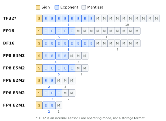
Figure 8-3. Reduced-Precision Formats for Deep Learning
| Format | Bits (s/e/m) | Largest finite | CUDA type | Introduced |
|---|---|---|---|---|
half |
1/5/10 | 65504 | __half |
(see Section 8.3.4) |
bfloat16 |
1/8/7 | 3.39×1038 | __nv_bfloat16 |
Ampere, CUDA 11.0 |
TF32 |
1/8/10 | (internal) | Tensor Core mode | Ampere |
FP8 E4M3 |
1/4/3 | 448 | __nv_fp8_e4m3 |
Hopper/Ada, CUDA 11.8 |
FP8 E5M2 |
1/5/2 | 57344 | __nv_fp8_e5m2 |
Hopper/Ada, CUDA 11.8 |
FP6 E2M3 |
1/2/3 | 7.5 (block-scaled) | __nv_fp6_e2m3 |
Blackwell, CUDA 12.8 |
FP6 E3M2 |
1/3/2 | 28 (block-scaled) | __nv_fp6_e3m2 |
Blackwell, CUDA 12.8 |
FP4 E2M1 |
1/2/1 | 6 (block-scaled) | __nv_fp4_e2m1 |
Blackwell, CUDA 12.8 |
Table 8-13. Reduced-precision floating point formats.
Two closing observations. First, these formats are not
general-purpose arithmetic formats: they are purpose-built for
processing by Tensor Cores, and a program reaches that processing not by
emitting matrix-multiply instructions by hand but by handing the
operands and their per-block scale factors to a library GEMM – cuBLASLt
(cublasLtMatmul) or CUTLASS. Second, the conversion
walkthrough in Appendix B applies to every row of the table – each
format is the same sign/exponent/mantissa story with different bit
budgets, and working through its float-to-half
converter (Listing B-1) equips you to reason about any of them.
| Format | Largest finite | Smallest normal | Smallest subnormal | Inf / NaN |
|---|---|---|---|---|
half (E5M10) |
65504 | 2-14 | 2-24 | yes |
bfloat16 (E8M7) |
3.39×1038 | 2-126 | 2-133 | yes |
FP8 E4M3 |
448 | 2-6 | 2-9 | NaN only |
FP8 E5M2 |
57344 | 2-14 | 2-16 | yes |
FP6 E2M3 |
7.5 | 1 | 2-3 | none |
FP6 E3M2 |
28 | 2-2 | 2-4 | none |
FP4 E2M1 |
6 | 1 | 2-1 | none |
Table 8-14. Extreme values of the reduced-precision formats. TF32, an
internal Tensor Core mode rather than a stored format, has
half’s precision with float’s range.
CUDA includes a built-in math library modeled on the C runtime
library, with a few small differences: CUDA hardware does not include a
rounding mode register (instead, the round mode is encoded on a
per-instruction basis15), so functions such as rint() that
reference the current rounding mode always round-to-nearest.
Additionally, the hardware does not raise floating point exceptions;
results of aberrant operations, such as taking the square root of a
negative number, are encoded as NaNs.
Table 8-15 gives the math library functions and the maximum error in ulps for each function. Most functions that operate on float have an “f” appended to the function name – for example, the functions that compute the sine function are as follows:
double sin( double angle );
float sinf( float angle );
These are denoted in Table 8-15 as e.g. sin[f].
| Ulp error | ||||
|---|---|---|---|---|
| Function | Operation | Expression | 32 | 64 |
| x+y | Addition | x+y | 01 | 0 |
| x*y | Multiplication | x*y | 01 | 0 |
| x/y | Division | x/y | 22 | 0 |
| 1/x | Reciprocal | 1/x | 12 | 0 |
| acos[f](x) | Inverse cosine | \(\cos^{- 1}x\) | 3 | 2 |
| acosh[f](x) | Inverse hyperbolic cosine | \(\ln\left( x + \sqrt{x^{2} + 1} \right)\) | 4 | 2 |
| asin[f](x) | Inverse sine | \(\sin^{- 1}x\) | 4 | 2 |
| asinh[f](x) | Inverse hyperbolic sine | \(sign(x)\ln\left( |x| + \sqrt{1 + x^{2}} \right)\) | 3 | 2 |
| atan[f](x) | Inverse tangent | \(\tan^{- 1}x\) | 2 | 2 |
| atan2[f](y,x) | Inverse tangent of y/x | \(\tan^{- 1}\left( \frac{y}{x} \right)\) | 3 | 2 |
| atanh[f](x) | Inverse hyperbolic tangent | \(\tanh^{- 1}x\) | 3 | 2 |
| cbrt[f](x) | Cube root: | \(\sqrt[3]{x}\) | 1 | 1 |
| ceil[f](x) | “Ceiling”, nearest integer greater than or equal to x | \(\left\lceil x \right\rceil\) | 0 | |
| copysign[f](x,y) | Sign of y, magnitude of x | n/a | ||
| cos[f](x) | Cosine | \(\cos x\) | 2 | 1 |
| cosh[f](x) | Hyperbolic cosine | \(\frac{e^{x} + e^{- x}}{2}\) | 2 | |
| cospi[f](x) | Cosine, scaled by π | \(\cos{\pi x}\) | 2 | |
| erf[f](x) | Error function | \(\frac{2}{\pi}\int_{0}^{x}{e^{{- t}^{2}}dt}\) | 3 | 2 |
| erfc[f](x) | Complementary error function | \(1 - \frac{2}{\pi}\int_{0}^{x}{e^{{- t}^{2}}dt}\) | 6 | 4 |
| erfcinv[f](y) | Inverse complementary error function | Return x for which y=1-erff(x) | 7 | 8 |
| erfcx[f](x) | Scaled error function | \(e^{x^{2}}\)(erff(x)) | 6 | 3 |
| erfinv[f](y) | Inverse error function | Return x for which y=erff(x) | 3 | 5 |
| exp[f](x) | Natural exponent | \(e^{x}\) | 2 | 1 |
| exp2[f](x) | Exponent (base 2) | \(2^{x}\) | 2 | 1 |
| exp10[f](x) | Exponent (base 10) | \(10^{x}\) | 2 | 1 |
| expm1[f](x) | Natural exponent, minus one | \(e^{x} - 1\) | 1 | 1 |
| fabs[f](x) | Absolute value | \(|x|\) | 0 | 0 |
| fdim[f](x,y) | Positive difference | \(\left\{ \begin{array}{r} x - y,x > y \\ + 0,\ x \leq y \\ NAN,x\ or\ y\ NaN \end{array} \right.\) | 0 | 0 |
| floor[f](x) | “Floor”, nearest integer less than or equal to x | \(\left\lfloor x \right\rfloor\) | 0 | 0 |
| fma[f](x,y,z) | Multiply-add | \(xy + z\) | 0 | 0 |
| fmax[f](x,y) | Maximum | \(\left\{ \begin{array}{r} x,x > y\ or\ isNaN(y) \\ y,otherwise \end{array} \right.\) | 0 | 0 |
| fmin[f](x,y) | Minimum | \(\left\{ \begin{array}{r} x,x < y\ or\ isNaN(y) \\ y,otherwise \end{array} \right.\) | 0 | 0 |
| fmod[f](x,y) | Floating point remainder | 0 | 0 | |
| frexp[f](x,exp) | Fractional component | 0 | 0 | |
| hypot[f](x,y) | Length of hypotenuse | \(\sqrt{x^{2} + y^{2}}\) | 3 | 2 |
| ilogb[f](x) | Get exponent | 0 | 0 | |
| isfinite(x) | Nonzero if x is not ±INF | n/a | ||
| isinf(x) | Nonzero if x is ±INF | n/a | ||
| isnan(x) | Nonzero if x is a NaN | n/a | ||
| j0[f](x) | Bessel function of the first kind (n=0) | \(J_{0}(x)\) | 93 | 73 |
| j1[f](x) | Bessel function of the first kind (n=1) | \(J_{1}(x)\) | 93 | 73 |
| jn[f](n,x) | Bessel function of the first kind | \(J_{n}(x)\) | * | |
| ldexp[f](x,exp) | Scale by power of 2 | \(x2^{\exp}\) | 0 | 0 |
| lgamma[f](x) | Logarithm of gamma function | \(\ln\left( \Gamma(x) \right)\) | 64 | 44 |
| llrint[f](x) | Round to long long | 0 | 0 | |
| llround[f](x) | Round to long long | 0 | 0 | |
| lrint[f](x) | Round to long | 0 | 0 | |
| lround[f](x) | Round to long | 0 | 0 | |
| log[f](x) | Natural logarithm | \(\ln x\) | 1 | 1 |
| log10[f](x) | Logarithm (base 10) | \(\log_{10}x\) | 3 | 1 |
| log1p[f](x) | Natural logarithm of x+1 | \(\ln(x + 1)\) | 2 | 1 |
| log2[f](x) | Logarithm (base 2) | \(\log_{2}x\) | 3 | 1 |
| logb[f](x) | Get exponent | 0 | 0 | |
| modff(x,iptr) | Split fractional and integer parts | 0 | 0 | |
| nan[f](cptr) | Returns NaN. | NaN | n/a | |
| nearbyint[f](x) | Round to integer. | 0 | 0 | |
| nextafter[f](x,y) | Returns the FP value closest to x in the direction of y. | n/a | ||
| normcdf[f](x) | Normal cumulative distribution | 6 | 5 | |
| normcdinv[f](x) | Inverse normal cumulative distribution | 5 | 8 | |
| pow[f](x,y) | Power function | \(x^{y}\) | 8 | 2 |
| rcbrt[f](x) | Inverse cube root | \(\frac{1}{\sqrt[3]{x}}\) | 2 | 1 |
| remainder[f](x,y) | Remainder | 0 | 0 | |
| remquo[f](x,y,iptr) | Remainder (also returns quotient) | 0 | 0 | |
| rsqrt[f](x) | Reciprocal | \(\frac{1}{\sqrt{x}}\) | 2 | 1 |
| rint[f](x) | Round to nearest int | 0 | 0 | |
| round[f](x) | Round to nearest int | 0 | 0 | |
| scalbln[f](x,n) | Scale x by 2n (n is long int) | \(x2^{n}\) | 0 | 0 |
| scalbn[f](x,n) | Scale x by 2n (n is int) | \(x2^{n}\) | 0 | 0 |
| signbit(x) | Nonzero if x is negative | n/a | 0 | |
| sin[f](x) | Sine | \(\sin x\) | 2 | 1 |
| sincos[f](x,s,c) | Sine and cosine | *s=sin(x); *c=cos(x); |
2 | 1 |
| sincospi[f](x,s,c) | Sine and cosine | *s=sin(πx); *c=cos(πx); |
2 | 1 |
| sinh[f](x) | Hyperbolic sine | \(\frac{e^{x} - e^{- x}}{2}\) | 3 | 1 |
| sinpi[f](x) | Sine, scaled by π | \(\sin{\pi x}\) | 2 | 1 |
| sqrt[f](x) | Square root | \(\sqrt{x}\) | 35 | 0 |
| tan[f](x) | Tangent | \(\tan x\) | 4 | 2 |
| tanh[f](x) | Hyperbolic tangent | \(\frac{\sinh x}{\cosh x}\) | 2 | 1 |
| tgamma[f](x) | True gamma function | \(\Gamma(x)\) | 11 | 8 |
| trunc[f](x) | Truncate (round to integer toward zero) | 0 | 0 | |
| y0[f](x) | Bessel function of the second kind (n=0) | \(Y_{0}(x)\) | 93 | 73 |
| y1[f](x) | Bessel function of the second kind (n=1) | \(Y_{1}(x)\) | 93 | 73 |
| yn[f](n,x) | Bessel function of the second kind | \(Y_{n}(x)\) | ** |
* For the Bessel functions jnf(n,x) and jn(n,x), for n=128 the maximum absolute error is 2.2×10⁻⁶ and 5×10-12, respectively.
** For the Bessel function ynf(n,x), the error is \(\left\lceil 2 + 2.5n \right\rceil\) for \(|x| < n\); otherwise the maximum absolute error is 2.2×10⁻⁶ for n=128. For yn(n,x), the maximum absolute error is 5×10-12.
1 On SM 1.x class hardware, the precision of addition and multiplication operation that are merged into FMAD instructions will suffer, due to truncation of the intermediate mantissa.
2 On SM 2.x and later hardware, developers can reduce this error rate
to 0 ulps by specifying --prec-div=true.
3 For float, the error is 9 ulps for |x|<8, otherwise the maximum absolute error is 2.2×10⁻⁶. For double, the error is 7 ulps for |x|<8, otherwise the maximum absolute error is 5×10-12.
4 The error for lgammaf() is greater than 6 inside the interval
-10.001, -2.264. The error for lgamma() is greater than 4 inside the
interval -11.001, -2.2637.
5 On SM 2.x and later hardware, developers can reduce this error rate
to 0 ulps by specifying --prec-sqrt=true.
Table 8-15. Math Library
According to the C runtime library definition, the nearbyint() and
rint() functions round a floating point value to the nearest integer
using the “current rounding direction,” which in CUDA is always
round-to-nearest-even. In the C runtime, nearbyint() and rint() differ
only in their handling of the INEXACT exception; but since CUDA does not
raise floating point exceptions, the functions behave identically.
round() implements “elementary school” style rounding: for floating
point values halfway between integers, the input is always rounded away
from zero. NVIDIA recommends against using this function because it
expands to eight (8) instructions as opposed to one for rint() and its
variants.
trunc() truncates or “chops” the floating point value, rounding
toward zero. It compiles to a single instruction.
float frexpf(float x, int *eptr);
frexpf() breaks the input into a floating point significand in the
range [0.5, 1.0) and an integral exponent for 2, such that:
\[x = Significand \bullet 2^{Exponent}\]
float logbf( float x );
logbf() extracts the exponent from x and returns it as a
floating-point value. It is equivalent to floorf(log2f(x)), except it is
faster. If x is a denormal, logbf() returns the exponent that x would
have if it were normalized.
float ldexpf( float x, int exp );
float scalbnf( float x, int n );
float scalblnf( float x, long n );
ldexpf(), scalbnf() and scalblnf() all compute \(x2^{n}\) by direct manipulation of floating
point exponents.
modff() breaks the input into fractional and integer parts:
float modff( float x, float *intpart );
The return value is the fractional part of x, with the same sign.
remainderf(x,y) computes the floating point remainder of dividing x by y. The return value is x-n*y, where n is x/y, rounded to the nearest integer. If \(|x - ny| = 0.5\), n is chosen to be even.
float remquof(float x, float y, int *quo);
Computes the remainder and passes back the lower bits of the integral quotient x/y, with the same sign as x/y.
The Bessel functions of order n relate to the differential equation:
\[x^{2}\frac{d^{2}y}{dx^{2}} + x\frac{dy}{dx} + \left( x^{2} - n^{2} \right)y = 0\]
n can be a real number, but for purposes of the C runtime, it is a nonnegative integer.
The solution to this second-order ordinary differential equation combines Bessel functions of the first kind and of the second kind:
\[y(x) = c_{1}J_{n}(x) + c_{2}Y_{n}(x)\]
The math runtime functions jn[f]() and yn[f]() compute \(J_{n}(x)\ \)and \(Y_{n}(x)\), respectively. j0f(), j1f(),
y0f(), and y1f() compute these functions for the special cases of n=0
and n=1.
The gamma function Γ is an extension of the factorial function, with its argument shifted down by 1, to real numbers. It has a variety of definitions, one of which is as follows:
\[\Gamma(x) = \int_{0}^{\infty}{e^{- t}t^{x - 1}dt}\]
The function grows so quickly that the return value loses precision
for relatively small input values, so the library provides the lgamma()
function, which returns the natural logarithm of the gamma function, in
addition to the tgamma() (“true gamma”) function.
Goldberg’s survey (with the captivating title “What Every Computer Scientist Should Know About Floating Point Arithmetic”) is a good introduction to the topic.
http://download.oracle.com/docs/cd/E19957-01/806-3568/ncg_goldberg.html
Nathan Whitehead and Alex Fit-Florea of NVIDIA have co-authored a white paper entitled “Precision & Performance: Floating Point and IEEE 754 Compliance for NVIDIA GPUs.”
http://developer.download.nvidia.com/assets/cuda/files/NVIDIA-CUDA-Floating-Point.pdf
Dekker and Kahan developed methods to almost-double the effective precision of floating-point hardware using pairs of numbers, in exchange for a slight reduction in exponent range (due to intermediate underflow and overflow at the far ends of the range). Some papers on this topic include:
Dekker, T.J. A floating-point technique for extending the available precision. Numer. Math. 18 (1971), pp. 224-242.
Linnainmaa, S. Software for doubled-precision floating point computations. ACM TOMS 7, 272-283 (1981).
Shewchuk, J.R. Adaptive precision floating-point arithmetic and fast robust geometric predicates. Discrete & Computational Geometry 18:305-363, 1997.
Some GPU-specific work on this topic has been done by Andrew Thall and Da Graça and Defour:
Da Graça Guillaume and David Defour. Implementation of float-float operators on graphics hardware, 7th Conference on Real Numbers and Computers, RNC7 (2006).
http://hal.archives-ouvertes.fr/docs/00/06/33/56/PDF/float-float.pdf
Thall, Andrew. Extended-precision floating-point numbers for GPU computation. 2007.
http://andrewthall.org/papers/df64_qf128.pdf
With the exception that single-precision denormals are not supported on SM 1.x hardware.↩︎
Sometimes called subnormals.↩︎
In fact, GPUs had full 32-bit floating point support before they had full 32-bit integer support. As a result, some early GPU computing literature explained how to emulate integers with floating point hardware!↩︎
Lindholm, Erik, John Nickolls, Stuart Oberman, and John Montrym. NVIDIA Tesla: A unified graphics and computing architecture. IEEE Micro, March-April 2008, p 47.↩︎
Note: half floating point values are supported as a
texture format, in which case the TEX intrinsics return float vectors
and the conversion is automatically performed by the texture hardware.↩︎
Encoding a round mode per instruction and keeping it in a control register are not irreconcilable. The Alpha processor had a 2-bit encoding to specify the round mode per instruction, one setting of which was to use the rounding mode specified in a control register! CUDA hardware just uses a 2-bit encoding for the four round modes specified in the IEEE specification.↩︎